Jul 19, 2024 - 7 min
Huber Loss
In machine learning, handling outliers effectively is crucial for building robust models. Traditional loss functions like Mean Squared Error (MSE) can be overly sensitive to outliers, while Mean Absolute Error (MAE) may not provide smooth gradients for optimization. Enter Huber Loss—a powerful alternative that blends the best of both worlds. By switching between squared and absolute loss based on a threshold
What is Huber Loss?
Huber loss combines the best of Mean Squared Error (MSE) and Mean Absolute Error (MAE).
Huber Loss is a piecewise loss function typically used in regression. It’s a mix of squared loss and absolute loss. For smaller errors, it behaves like a squared loss providing smooth gradients and for larger errors it behaves as absolute loss, reducing the impact of outliers. Its particularly useful for tasks containing outliers.
Huber loss provides robustness by switching to absolute loss when the error term crosses a predefined threshold/parameter
Samples for which the
Huber Loss Formulation
Huber Loss is defined as such
where, parameter
You’ll notice that when
Below is the graph we get if we simply switch to
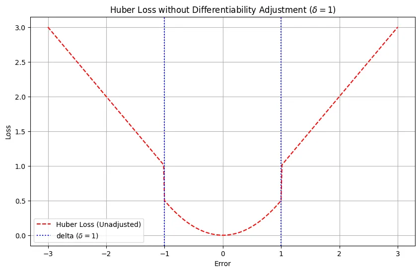
Huber Loss when we don’t ensure differentiability
Its clear from the graph above that a simple switch wont give us a smooth differentiable function. In order to ensure differentiability let us first calculate the value of the squared loss when
We substitute
For the loss to be smooth throughout, we need to ensure that our loss functions returns
for larger errors
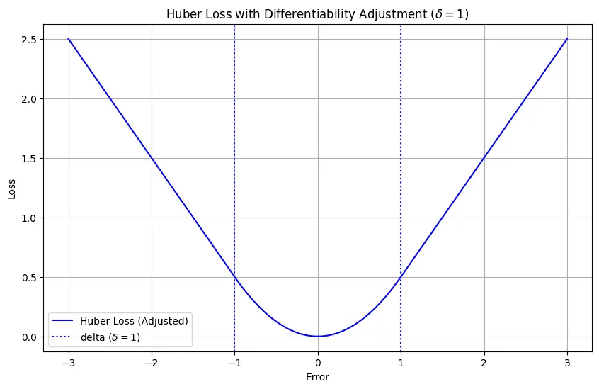
Huber Loss after we modify the absolute loss to ensure differentiability
Gradient of Huber Loss
The gradient of the Huber loss with respect to the predictions comes out to be
If you see the loss term for cases when
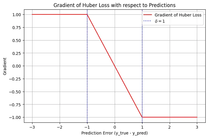
The Huber loss caps the loss for outliers which prevents outsized adjustments to the weights. This helps reducing the model’s sensitivity to outliers.
Properties
- Combination of
and loss: Huber loss is for smaller losses and for larger losses. It ends up penalizes smaller errors strongly compared to larger losses - Convexity: Huber Loss is a convex function which means it is well suited for gradient optimization as it can converge to global minima effectively without getting stuck at a local minima
- Differentiability: Huber Loss is differentiable everywhere. The transition from square to linear is smooth ensuring continuous first derivatives
- Robustness to Outliers: Huber Loss is designed to be robust against outliers. It achieves this by capping the loss for large loss terms
- The
Parameter: The parameter is the point where the loss switches from quadratic to linear. Tuning the parameter allows for adjusting the model’s sensitivity towards outliers. If is large then the model tends towards being squared loss heavy. If is small then it leans towards being more of an absolute loss Choosing a suitable is important. Too large values will fail to mitigate the impact of outliers. Too small and it may overly desensitize the model and cause underfitting.
How to select Delta?
Selecting
- Compute
for all training points - Pick
as 75th, 90th, or 99th percentile to cover most inliers while treating the tail as outliers - You can also pass
as a hyperparameter to be tuned and selected
Further Reading
- Huber Regressor
- Huber Loss – Loss function to use in Regression when dealing with Outliers
- The Huber Loss Function And Its Application
Read more here