Statistical Testing 101 | shubham's notes

In the era of LLMs, AI agents, and other groundbreaking technologies, one essential concept holds its ground—statistical testing. It serves as the foundation for many companies when evaluating whether a new feature or model resonates with their users. In this post, we’ll dive into Statistical Testing 101 to explore some of the key tests in the field.

The Underlying Structure

Multiple attempts later of learning and trying to remember these test formulas, I felt there had to be a simpler way. There has to be a pattern to these formulas that could make them easier to remember. After tinkering around, I can comfortably say that common statistical tests follow the below pattern

$Missing argument for \text\text\{Test Statistic\} = \frac\{\text\{Estimate\} – \text\{Null Value\}\}\{\text\{Standard Error\}\}$

Once we calculate this statistic, we compare it with the appropriate distribution(). Knowing that statistical tests tend to follow the above structure, helped me understand them clearly and more intuitively.

We will discuss how to select the appropriate test statistic based on the sample parameter we want to test and the distribution of our data. But first, let’s look at some commonly used tests.

Commonly Used Statistical Tests

Z-Test

Z-test is commonly used for comparing proportions. There are two types of Z-tests: one proportion and two proportion. The aim of these tests is

one proportion: it evaluates if the proportion of a single sample differs from a known benchmark proportion. Example: Is the proportion of repeat customers equal to 60%?
two proportion: it compares the proportions from two different samples to determine if they differ significantly. Example: Is the proportion of satisfied customers from Store A the same as that from Store B?

The null hypothesis () for both cases is: The two proportions are equal ( or )

The alternate hypothesis () for both cases is: The two proportions are not equal ( or )

The one-proportion test compares a single sample to a benchmark value, whereas the two-proportion test compares two independent samples to see if their proportions are statistically different.

The formula for two proportion Z-Test is

where the pooled proportion is given by:

and

is the proportion in group 1,
is the proportion in group 2,
are the number of successes in each group,
are the sample sizes of each group.

Deriving the One Proportion Z-Test Formula

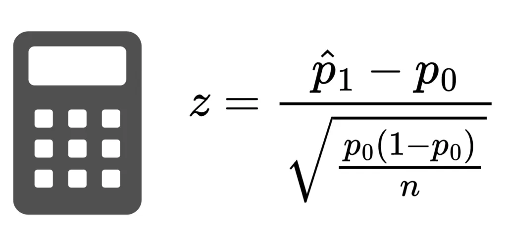
If you are wondering what the formula for one proportion Z-test is– let us start by considering to be infinite. Since is infinite, it is a population parameter now- we’ll call it . Due to being infinite, the pooled proportion will become

due to being infinite and go to zero and we are left with which is . So we can say that as , we get . Ultimately the formula comes down to

Compare the two formulas to the structure formula given in the first section! The numerator in both the formulas is easy to observe– they follow the format. The denominator is the standard error, which is calculated as shown above for proportions.

T-Test

The T-Test also has two variants- similar to the Z-Test. The T-Test is used to compare the mean of a sample to either

a benchmark value
the mean of another sample

The null hypothesis () for both cases is: The means are equal ( or )

The alternate hypothesis () for both cases is: The means are not equal ( or )

Alright, let’s look at the formulas. Remember the underlying structure we talked about initially and see if the formulas fit the structure.

$Missing argument for \bart = \frac\{\bar\{x\}_1 – \bar\{x\}_2\}\{s_p \sqrt\{\frac\{1\}\{n_1\} + \frac\{1\}\{n_2\}\}\}$

where:

is the pooled standard deviation given by:
and are the sample means for groups 1 and 2
and are the sample sizes

Degrees of Freedom

You may have already noticed a new addition to the formula- . What is that? stands for degrees of freedom. Conceptually, degrees of freedom have the same meaning as its literal definition. It is the number of “free choices” we have when calculating a statistic.

Imagine, we have the choice to select 5 numbers. But no matter what we choose, the total must be 100. For the first four numbers, we are free to choose whatever values we like. The last number, however, will be governed by 100- total so far to get to the full 100. Here we have no freedom.

In statistical tests, the degree of freedom represents the number of independent observations that we can use to estimate the parameter after accounting for the constraints. It’s a way of counting how many values can vary on their own, which is crucial for determining the reliability and variability of your estimates.

When we have higher , we have a lot of independent observations. This means we have a fairly large sample size. With higher , our estimates are more reliable, and we get narrower confidence intervals (more on this later)

On the other hand, lower implies we have a smaller dataset. As a result, we have to deal with less reliable estimates and wider confidence intervals.

Decision Making

So far, we have looked at the Z-Test and T-Test and its variants. But what do we do after calculating the z-score and the t-score? How do we make a decision?

We use the calculated scores to decide whether to reject the null hypothesis or fail to reject it.

Significance Level

Well, we need one more piece of information before making a decision. We need to set the significance level for our tests. What does this abomination mean? Simply said, it is the maximum risk we are willing to accept that we mistakenly reject the null hypothesis

That’s weird, right? Why would we want to take any risk while making decisions? Why not just take no risk in our decision-making? I understand the sentiment and it seems the ideal thing to do. But in statistics, we usually deal with sampled data, we don’t have access to the entire population. This introduces uncertainty, which means we need to adapt our methods. By choosing a significance level, we are taking on a controlled risk. To eliminate risk completely, we would need complete information about the population, at that point, making a decision would be pointless.

Significance Level is usually represented as in statistical testing. For a given significance level, we find the critical value using the appropriate distribution (more on this later, but this depends on the test we are conducting). If the absolute value of our t-score or z-score is greater than the critical value, we reject the null hypothesis. If the test statistic does not exceed the critical value, we fail to reject the null hypothesis

Critical Values and p-values

In hypothesis testing, two concepts help us decide whether to reject the null hypothesis or whether to accept it.

Critical values define the threshold beyond which the test statistic is considered extreme enough to reject the null hypothesis. These values depend on the chosen significance level (). It also depends on the sampling distribution of the test statistic. In a test at , the critical value for a z-test is approximately . If the absolute value of the calculated z-score exceeds this value, we reject the null hypothesis.

p-value tells us how probable it is to observe a calculated score as extreme as ours even if the null hypothesis is true. Let’s say someone claims that the average height of men in a town is 160cm. You take a sample of the city men and calculate the mean height, which comes to 190 cm. At , you get a p-value of 0.0001. This implies that if the true average was 160 cm, there is a 0.01% chance that the difference is purely due to chance.

A small p-value (typically less than ()) indicates strong evidence against (), leading us to reject it. Conversely, a large p-value suggests that the observed result is consistent with the null hypothesis.

Caveat: people often interpret the p-value as the probability of the null hypothesis being true. That is incorrect. p-value is the probability of getting a deviation as extreme as ours assuming the null hypothesis is true.

What does the Z-score and the T-score measure?

We have discussed a lot, but we haven’t yet touched on one important aspect. We calculate these scores, but what do they measure? They are measures of extremeness. When these values are close to zero, the observed values are in line with our null hypothesis. The larger the gap between the sample mean(or proportion) and the other sample/benchmark value, the higher these scores will be.

Going back to the initial formula we discussed:

$Missing argument for \text\text\{Test Statistic\} = \frac\{\text\{Estimate\} – \text\{Null Value\}\}\{\text\{Standard Error\}\}$

Take a look at the numerator– the larger the gap, the larger the score, and the more extreme the difference between the two values.

There is a second part to this equation– the denominator. The Standard Error is usually calculated as:

Hiding in the denominator of SE is which represents the sample size. The larger the sample size, the smaller the SE becomes. For the same difference in the numerator, a larger sample size results in a smaller SE. This leads to larger test scores, making the difference more extreme.

Conclusion

In this Statistical Testing 101 post, we explored the underlying structure common to many statistical tests, delved into the formulas for z-tests and t-tests (and their variants), and discussed how to interpret test statistics, p-values, and critical values. While we’ve covered many essential topics, there is still much to learn—including assumptions, effect sizes, power analysis, and more nuanced interpretations of p-values. Stay tuned for Part 2, where we’ll dive deeper into these advanced topics and explore additional testing scenarios.

That’s it on Statistical Testing 101 for today! Stay tuned, keep reading!