Multi-Head vs Multi-Query vs Grouped Query Attention

The title may be long, but the explanation isn’t. Since the original Transformer, researchers have continuously tweaked its architecture, aiming to cut inference costs. Today, we’ll compare Multi-Head vs Multi-Query vs Grouped Query Attention to understand these innovations better.

Note: This article assumes you’re familiar with self-attention. If you’re new to this concept, consider reading this gentle but comprehensive introduction.

The Usual Suspect 🥁🥁 – Attention

Since ChatGPT’s explosive adoption, developers have increasingly looked for ways to optimize model architecture to curb massive inference expenses. As models scale up, the computational and inference demands escalate significantly.

It’s no surprise that teams quickly turned their attention to the main culprit: Attention.

Attention in LLMs scales quadratically with sequence length. In simpler terms, as context grows, generating each additional token gets disproportionately more expensive. Researchers have proposed various strategies-from memory management to hardware optimizations. Among these, Multi-Query Attention and Grouped Query Attention are promising alternatives to the traditional Multi-Head Attention.

But first, let’s briefly revisit Multi-Head Attention…

Multi-Head Attention (MHA)

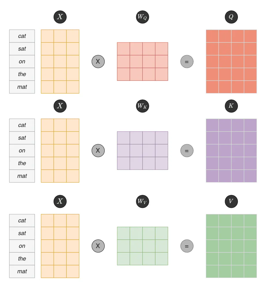
Fig. 1: The input embedding matrix is linearly mapped via , , and to produce the Query (), Key (), and Value () matrices used in the attention calculation

The diagram above illustrates the core mechanism of an attention head. Each token is projected into query, key, and value vectors. The query and key vectors are multiplied (followed by scaling, though we’ll skip that detail here) to compute attention scores. These scores are then used to weight the value vectors, producing each head’s attention output. Crucially, every attention head has its own projection matrices—, , and . For instance, the LLaMA-3.1 70B model employs 64 attention heads per layer.

As models scale up (e.g., LLaMA-3.1 405B has 128 heads), the number of heads increases along with computational costs. Typically, when a model mentions “H attention heads,” it refers to the count per layer.

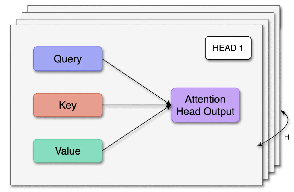
Fig. 2. Multi-Head Attention runs H parallel attention heads—each mapping a Query, Key, and Value to an “Attention Head Output”—then concatenates all head outputs to form the final representation.

There’s more intricacy within attention heads, but for our current discussion, we need to note that in MHA, each head maintains distinct projection matrices.

Multi-Query Attention (MQA)

While MHA is powerful, its computational cost is steep due to individual projection matrices per head.

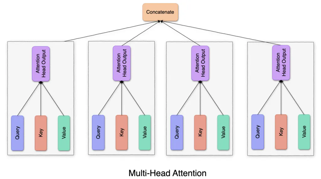
Fig. 3: Each head independently applies query, key, and value projections, then concatenates results to capture diverse subspaces

Multi-Query Attention aims to reduce this computational overhead. Instead of separate key/value projections for every head, MQA proposes using a shared set of key/value projection matrices (, ) per layer, while each head retains a unique query projection matrix ().

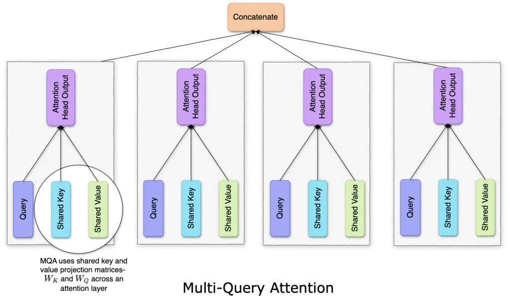
Fig. 4: All heads share a single pair of key/value projection matrices (, ); each head maintains its unique query projection, significantly cutting down parameters.

So the major difference from MHA to MQA is the sharing of the and the matrices. Looking at the image, the number of computation steps appears to be the same, so how do we save on computation if we are doing the same number of steps? Instead of calculating and multiple times for each attention head, we compute them just once per layer. This brings down the number of compute steps required to calculate the attention outputs.

Speed and Quality

This compute saving, however, comes at an obvious cost– degradation of output quality. But first, let’s look at the speed gains we get because they are extremely encouraging

MQA Speed Gains on WMT’14 – Decoder-only per token: 46 µs → 3.8 µs (×12) – Greedy end-to-end: ~48 µs → ~5 µs (×9) – Beam-4 search: ~205 µs → ~33 µs (×6) Source

MQA Performance on WMT’14 – Perplexity (dev): 1.424 → 1.439 (+1%) – BLEU (dev, beam 1): 26.7 → 26.5 (-0.2) – BLEU (test, beam 4): 28.4 → 28.5 (+0.1) Source

Grouped-Query Attention (GQA)

On one hand, we have MHA, which trains unique , matrices per layer ( is the number of attention heads per layer), and on the other hand, we have MQA, which uses just one and matrix per layer. GQA is a variant that aims to balance the two by keeping the number of projection matrices- and anywhere between to per layer. We can view GQA as a generalization with MHA and MQA being extremes.

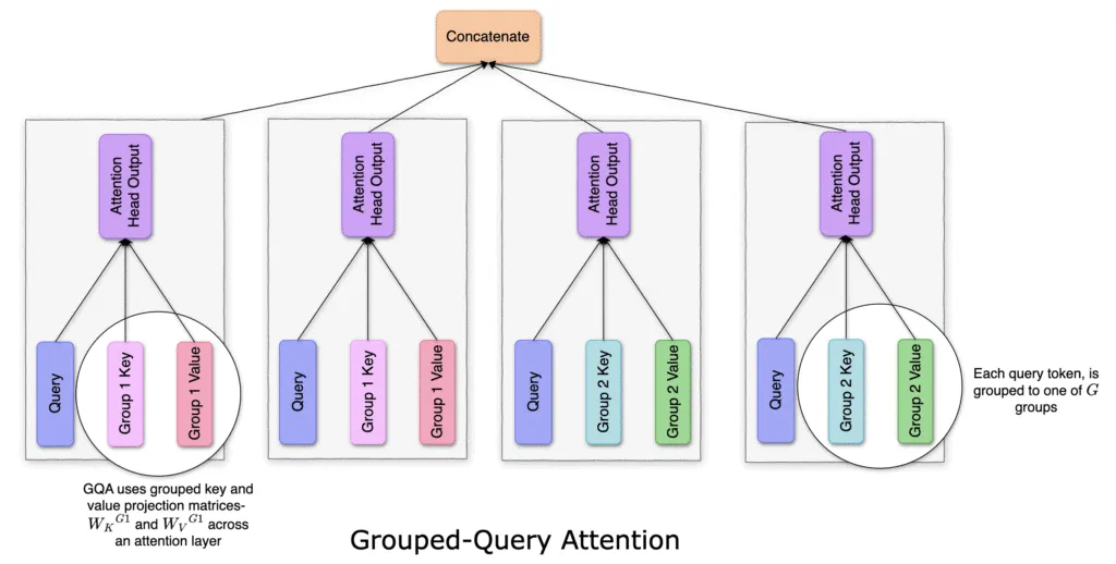
Fig. 5: The model uses query projections to attend grouped key/value subspaces and concatenates the resulting attention outputs, yielding multi-head expressivity with far fewer parameters.

In GQA, we divide H attention heads into G groups, each sharing key/value projections. Specifically, if G=1, we revert to MQA, and if G=H, we have MHA. Tokens are projected into H queries, then grouped into G subsets. Within each subset, queries share key/value matrices, reducing computational steps by a factor of H/G.

Heads are deterministically partitioned: heads 0 through (H/G−1) belong to group 1, heads H/G through (2H/G−1) form group 2, and so forth.

Developers have widely adopted GQA across models since its release. Meta integrated it into the Llama 3 series (2024). Mistral AI adopted GQA for its 7B as well. Llama 3.3 and 4 series also use GQA.

"num_attention_heads": 32,
"num_hidden_layers": 32,
"num_key_value_heads": 8,

Snippet from the Mistral-7B-Instruct-v0.3 config

Multi-Head vs Multi-Query vs Grouped Query Attention

Model	Inference Time (ms)	Avg. Dev-Set Score
MHA-Large	0.37	46.0
MHA-XXL	1.51	47.2
MQA-XXL	0.24	46.6
GQA-8-XXL	0.28	47.1

The above comparison uses the T5-Large as the baseline. The baseline model using full multi-head attention (MHA) processes each sample in 0.37 ms while achieving an average dev-set score of 46.0.

Scaling up to the T5-XXL model with full MHA raises the average score to 47.2 but nearly quadruples latency to 1.51 ms per sample. Converting to a single shared key–value head (MQA-XXL) delivers the fastest inference at 0.24 ms per sample, although quality dips down to 46.6.

By setting G between these extremes with eight grouped key–value heads (GQA-8-XXL), the model achieves a near-MQA throughput of 0.28 ms per sample while recovering almost all the performance of the large MHA model, scoring 47.1, just 0.1 points below MHA-XXL.

Conclusion

MHA sets the quality benchmark but incurs high inference costs. MQA drastically cuts latency by sharing key/value projections across heads, slightly compromising quality (by 1–2%). GQA offers a middle ground, capturing MHA’s quality at near-MQA speeds and minimal extra training cost (~5%). Production adoption in LLaMA-3 and Mistral-7B underscores GQA’s practicality.

In short: Choose MHA for peak accuracy, MQA for maximum speed, and GQA for the optimal balance of both.